A Matrix for Numerical Integration

My very small addition to the field of Numerical Analysis

I’m working on algorithmically generating bicycle parts. In order to optimize the geometry, I’ve had to solve some differential equations numerically. Some of the solution techniques require fairly accurate numerical integration, or quadrature,  but typical quadrature techniques like gaussian quadrature won’t work because they require irregularly spaced samples.

For the numerical differentiation, I’m using finite difference matrices with fourth order accuracy, and I’d like to be able to use a simple matrix multiplication for the numerical integration as well. 

Simpson’s rule seems like the obvious next choice for numerical integration because it’s relatively simple, it’s reasonably accurate (4th order) and it works on data with equal spacing.

Simpson’s method is good for integrating a whole vector, but I want a cumulative sum, a numerical anti-derivative matrix. The numerical differentiation matrices I’m using spit out a vector, so there seems to be no reason why I can’t create a matrix that, when multiplied by a vector, returns the antiderivative of that vector. After poking around on the internet for a few hours, I was not able to find any sort of cumulative simpson’s rule matrix which was puzzling.I knew that it must be possible so I went ahead and derived my own. 

Because a cumulative integral would necessarily have to be a weighted sum of the previous values of a vector, this matrix would have to be a sort of lower triangular matrix. With this in mind, I chased a few dead ends and ended up finding a link to this brilliant paper buried deep in the scipy quadrature source code. https://www.msme.us/2017-2-1.pdf

The formulae for cumulative simpson’s rule are pretty straightforward and more elegant than I anticipated. It’s just two equations:

These two equations are super easy to code up in Python

def simpsons_rule_matrix(num_nodes):
    #I think I'm just going to use this:
    #https://www.msme.us/2017-2-1.pdf
    #build up the S matrix
    
    S = np.zeros((num_nodes,num_nodes))
    for k in range(num_nodes):
        if k ==0:
            pass
        elif k == 1:
            S[k,0:3] = np.array([1.25,2,-0.25])
        else:
            simps_stencil = np.zeros(k+1)
            simps_stencil[-3:] = np.array([1,4,1])
            S[k,0:k+1] = S[k-2,0:k+1] + simps_stencil
    return(S)

And now I have my integration matrix. Strangely enough, mine is the only implementation of the cumulative Simpson’s rule as a matrix multiplication that I could find. My own small contribution to the field of numerical analysis. I also wrote functions for creating finite difference matrices for the first and second derivatives of a vector. This calculator was very handy for calculating the coefficients for the finite differences matrices. My difference matrices are accurate to the 4th order as is my simpson’s rule matrix. These three matrices will come in handy for the algorithmically generated geometry project that I mentioned above. Here are the matrices in action: 

I plotted y=x^2 along with its first derivative, 2x, its second derivative, 2, and its integral, 1/3 x^3. 

Here are the residuals plotted. This is the numerical solution minus the analytic solution. It's dead on; error terms are on the order of 10^-14. But this is to be expected.

The astute reader may be thinking “you’re pulling a fast one on us, Jim. Simpson’s rule uses a parabolic fit, so you are using parabolas to interpolate a parabola. Of course it’s dead on!” And you’d be right. But to further prove that it works, here is another function, cosine, which is described by an infinite series of polynomials. (Calculate and plot the difference between the numeric solution and the algebraic solution.)

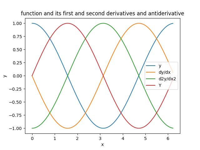
Here are the residuals for y = cos(x). I’m not getting the machine epsilon residuals I was seeing with y = x^2, but the residuals are on the order of 10^-7 for n = 100 which is pretty good.

Now that I have reasonably accurate matrices for taking the integral, the first derivative and the second derivative, there are some pretty neat calculations I can run.

The parts that I am algorithmically generating are somewhat round, so a polar coordinate system is the logical choice. Some of the constraints that I’m using require both integrals and derivates of the original function. Furthermore, I’m going to have to figure out how to add instantaneous slope and concavity constraints in polar coordinates. Luckily, the generous educators at Whitman College provided the formula for calculating both.  https://www.whitman.edu/mathematics/calculus_online/section10.02.html

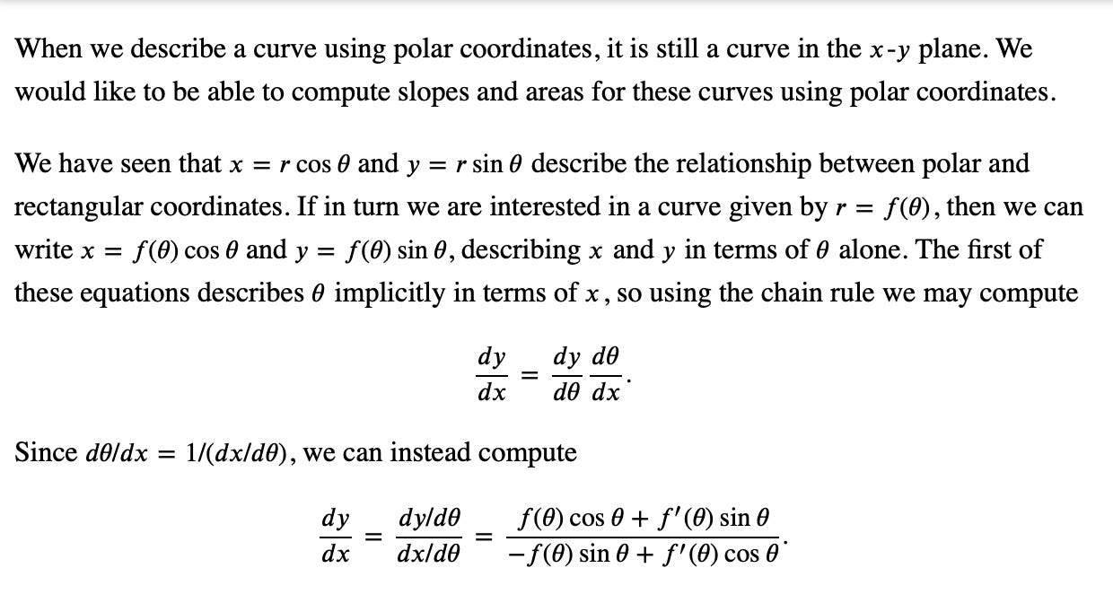
I can get the instantaneous slope and curvature of my curve in polar coordinates using some differentiation tricks. Here is a quick example: An oval in Polar coordinates.

Because its just an oval in the plane and the coordinate systems are simply different ways of describing the curve, I can plot the same oval in rectangular coordinates. It’s the exact same shape.

Now I have the radial dimension unrwapped and plotted against the angle. And I used my finite differences matrices and the formulae from Whitman college to calculate the instantaneous slope and curvature of the oval.

This plot is pretty interesting. The radius of the oval is plotted with respect to theta. The first derivative, the instantaneous slope of the oval, and the second derivative of the oval, the instantaneous curvature of the oval are plotted as well. The orange line is the dy/dx, the instantaneous slope of the oval. It makes sense when you trace your way around the oval. It starts out at negative infinity indicating a vertical line and then crosses the y axis at pi/2 on its way to positive infinity. The green line is the d^2y/dx^2 or the concavity of the oval. This function is a little less well behaved. I’d need to look at the closed form solution to the d^2y / dx^2, but I’d imagine that the denominator has something like a sin(1/x)/x that gets really unstable close to zero and pi in this case. Either way, the sign of the well-behaved portions of the function match my intuition (0,pi) has a negative sign indicating concave down and (pi, 2pi) has a positive sign indicating concave up. This matrix will be super helpful for my constrained optimization, but first I need to solve a few tricky differential equations.